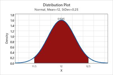
An engineer for a soda bottling facility collects data on soda can fill weights. The engineer determines that the fill weights follow a normal distribution with a mean of 12 ounces and a standard deviation of 0.25 ounces. The engineer analyzes the distribution of the data to determine the probability that a randomly chosen can of soda has a fill weight that is between 11.5 and 12.5 ounces.
- Choose .
- Select View Probability, then click OK.
- From Distribution, select Normal.
- In Mean, enter 12.
- In Standard deviation, enter 0.25.
- Click the Shaded Area tab.
- In Define Shaded Area By, select X value.
- Click the Middle icon. This option shows the probability that is between two x-values.
- In X value 1, enter 11.5. In X value 2, enter 12.5.
- Click OK.
Interpret the results
If the population of fill weights follows a normal distribution and has a mean of 12 and a standard deviation of 0.25, then the probability that a randomly chosen can of soda has a fill weight that is between 11.5 and 12.5 ounces is 0.9545.