What is a continuous distribution?
A continuous distribution describes the probabilities of the possible values of a continuous random variable. A continuous random variable is a random variable with a set of possible values (known as the range) that is infinite and uncountable.
Probabilities of continuous random variables (X) are defined as the area under the curve of its PDF. Thus, only ranges of values can have a nonzero probability. The probability that a continuous random variable equals some value is always zero.
Example of the distribution of weights
The continuous normal distribution can describe the distribution of weight of adult males. For example, you can calculate the probability that a man weighs between 160 and 170 pounds.
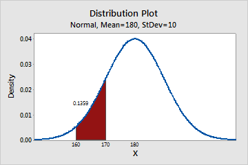
Distribution plot of the weight of adult males
The shaded region under the curve in this example represents the range from 160 and 170 pounds. The area of this range is 0.136; therefore, the probability that a randomly selected man weighs between 160 and 170 pounds is 13.6%. The entire area under the curve equals 1.0.
However, the probability that X is exactly equal to some value is always zero because the area under the curve at a single point, which has no width, is zero. For example, the probability that a man weighs exactly 190 pounds to infinite precision is zero. You could calculate a nonzero probability that a man weighs more than 190 pounds, or less than 190 pounds, or between 189.9 and 190.1 pounds, but the probability that he weighs exactly 190 pounds is zero.
What is a discrete distribution?
A discrete distribution describes the probability of occurrence of each value of a discrete random variable. A discrete random variable is a random variable that has countable values, such as a list of non-negative integers.
With a discrete probability distribution, each possible value of the discrete random variable can be associated with a non-zero probability. Thus, a discrete probability distribution is often presented in tabular form.
Example of the number of customer complaints
| x | P (X = x) |
|---|---|
| 5 | 0.037833 |
| 10 | 0.125110 |
| 15 | 0.034718 |
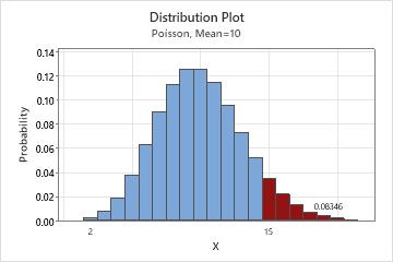
Distribution plot of the number of customer complaints
The shaded bars in this example represents the number of occurrences when the daily customer complaints is 15 or more. The height of the bars sums to 0.08346; therefore, the probability that the number of calls per day is 15 or more is 8.35%.